A consumer optimum represents a solution to a problem facing all individuals -- maximizing the satisfaction (utility) from consuming different goods and services subject to the constraint of household income and product prices. This problem can be described as follows:

max U = f(X,Y)

s.t. P_x(X) + P_y(Y) < I

In this problem, the objective function is unobservable leading to the use of assumptions about consumer preferences and diagrammed through the use of indifference curves. The slope of these indifference curves also known as the Marginal Rate of Substitution (MRS) represents the ratio of the marginal utilities of the two goods.

MRS^xy = MU_x/MU_y

The Budget Set / Budget Constraint

However, the all variables and parameters in the budget constraint are observable and thus in defining our consumer optimum, we assume that this optimum lies on this constraint. This budget constraint can be written in several ways. First we can write it as a budget set 'B':

B = {X,Y ε R² | X,Y > 0; P_x(X) + P_y(Y) < I₀}

This budget set represents all combinations of the two goods that are attainable to the consumer given his level of income and the the market-determined prices of these goods. Second, we can write it as a budget constraint expressed as an exact equality in intercept-slope form:

Y = I₀/P_y - (P_x/P_y)X

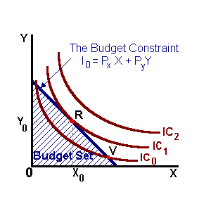
The slope of this budget constraint is a relative price (the price of good-x relative to the price of good-y) where a change in any price, either in absolute or relative terms, will lead to a rotation of this constraint. Both this budget constraint and budget set are shown in the figure below.

A Consumer Optimum

In this diagram, we can note that many bundles of 'x' and 'y' on IC₀ are within this budget set and thus attainable. However, any point in the interior of the budget set represents an inefficient use of income. Point V on this same indifference curve does represent an efficient use of income however, the consumer can do better. At this point the slope of the budget constraint is greater than the slope of the indifference curve...

P_x/P_y > MU_x/MU_y

or

MU_x/P_x < MU_y/P_y

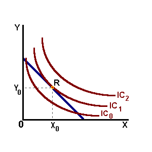
At this point the marginal utility per dollar spent on good-x is less that the marginal utility per dollar spent on good-y. This consumer can increase his level of satisfaction by reallocating his income to buy more of good-y (thus MU_y will decrease given our assumption of diminishing marginal utility) and buy less of good-x (MU_x increases). This reallocation of income can be seen as a movement along the budget constraint from point V to point R. It is at point R that the consumer has found an optimum on IC₁ where:

MU_x/MU_y = P_x/P_y

or

MRS^xy = P_x/P_y

This is our condition for a consumer optimum. Note that any bundle on IC₂, although providing a greater level of satisfaction, lies entirely beyond the budget set and thus could never include a solution to the problem facing the consumer.

Exogenous Shocks

Original Position Increase in Income. Decrease in Px. Decrease in Py.

In the figure above we can examine the effect of an increase in consumer income [click on the "Income (increase)" button. This change leads to a parallel outward shift in the budget constraint (the slope remains the same since relative prices have not changed). This increase in income increases the size of the budget set making a greater number of consumption bundles attainable to the consumer. This increase in the size of the budget set implies that the consumer will be better-off as defined with the new consumer optimum at point T. With this increase in income, the consumer chooses to consume both more of both goods indicating that they are both normal goods to that individual. It is possible that with this type of shock, the consumer will choose to purchase more of one good and less of the other (a movement from R to T in the northwest or southeast direction). In this case one good is normal and the other an inferior good. It must be true that at least one good in the consumption bundle is a normal good. If all goods were inferior, then an increase in income would lead to a consumer optimum in the interior of the budget set.

Additionally, we see the effects of changes in market price (click any of the appropriate buttons). In the case of a decrease in the price of good x)the budget line rotates outward and the price ratio declines (good-x is less expensive in absolute and relative terms, good-y is more expensive in relative terms). This outward rotation also leads to an increase in the size of the budget set such that the consumer should be better off. We find that with this particular price change, the consumer is buying more of good-x and more of good-y as defined by a new consumer optimum at point T.

The increase in the amount of good-x consumed is expected as it is now cheaper to the consumer. However the increase in consumption of good-y requires some explanation.

A change in the price of one particular good has two effects on consumer behavior. First, is the substitution effect where the consumer substitutes towards that good that is relatively cheaper (good-x) and away from that good that is relatively more expensive (good-y). Based on the substitution effect alone, we would expect the consumer to buy more of good-x and less of good-y. In the case of the latter good, this is not the case. A decrease in the price of any good in the consumption bundle also leads to an increase in purchasing power. The impact of this change is known as the income effect where, with this increase in purchasing power, the consumer will buy more normal goods and fewer inferior goods. In figure 3, we find that the consumer may be substituting away from good-y but he is also using the increase in purchasing power to actually buy more of that good.

Price Decomposition

Original Position A Price Change Decomposition Substitution Effect (R-S) Income Effect (S-T) Total Effect (R-T)

These two effects can be graphically decomposed from the price reduction. We define the substitution effect as a comparison of the old price ratio (Px/Py) and the new (Px*/Py) holding the level of utility constant. We can see this substitution effect in figure 4, by looking at the tangency of the original budget constraint (old price ratio) at point R and a different tangency on the same indifference curve IC₁ defined by the new price ratio at point S. The income effect is defined as a comparison between the two levels of satisfaction defined by IC₁ and IC₂ holding relative prices constant. Comparing the two levels of utility acts as a proxy for changes in purchasing power (similar to a change in the size of the budget set). This can be seen as the parallel shift from point S on IC₁ to point T on IC₂. We find in this example that the consumer is substituting towards good-x and away from good-y and, in addition, he is using the increase in purchasing power to buy more of both goods.

This decomposition in price helps in the understanding of the responsiveness of individual demand to changes in market price. For a price reduction, the consumer will always demand more of that good based on the substitution effect. However, the income effect will either augment demand for this good in the case of normal goods or offset some of this increase in demand in the case of inferior goods.

For example, if the good in question is a normal good, then a reduction in market price will lead to a healthy increase in quantity demanded. The larger the income effect, the greater the increase in quantity demanded for this good. The individual demand curve will be relatively flat (or relatively elastic). If the good in question is an inferior good, then a reduction in market price will have a smaller impact on demand. With this good being relatively cheaper the consumer will choose to buy more (the substitution effect). As purchasing power increases the consumer chooses to buy less (the income effect). These two effects working on opposite direction will lead to a smaller quantity demanded -- the individual demand curve will be relatively steep (relatively price inelastic). It could be the case that the income effect exactly offsets the substitution effect such that the observed change in quantity demanded (the Total Effect) is unchanged.