10.3.1 The Implementation of Monetary Policy

Expansionary Monetary policy may be used for the same reasons as expansionary fiscal policy - weak aggregate demand and an economy operating below its potential. The Federal Reserve will only be comfortable using this type of policy if there is little chance that inflation will not become a future problem (i.e., π = π^target ~ 2.0%).

In this situation, the Fed will use open market operations to purchase Government securities (bonds) from Treasury dealers paying for those securities with newly created reserves. (More recently, the Fed is buying other assets through Quantitative Easing). The Federal Reserve of N.Y. trading desk with the purchase of these securities, will put upward pressure on these bond prices thus driving their yield downward (Ψ ↓). These reserves finding their way into the banking system as excess reserves will be converted by bankers into new loans - loans available to borrowing customers at lower interest rates.

Before we model the relationship between monetary changes and changes in expenditure, we need to augment our expenditure equations (see module 4) to include the interest rate.

Consumption expenditure is given by:

C = C₀ + b(1 - t)Y

where 'C₀ represents autonomous expenditure, 'b' is the MPC and 't' is the Tax rate. Consumption is proportional to income.

If we modify the other expenditure categories such that we define investment as being inversely related to market interest rates:

I = I_o - h(r),

The parameter 'h' represents the interest sensitivity of investment.

Autonomous expenditure includes: Government spending and Net-Export spending

G = G₀, NX = X_o - M_o

where: 'G'₀' is autonomous government spending, 'X'₀' is autonomous export spending and 'M₀ represents autonomous import spending.

Summing the expenditure categories and solving for 'Y':

Y = C + I + G + NX

Y = Z₀ + b(1-t)Y - h(r)

given: Z₀ = C₀+ I₀+ G₀ + X₀ - M₀

or

Y [1 - b(1-t)] = Z₀ - h(r)

The spending multiplier α may be written as:

α' = 1/[1 - b(1 - t)]

and

Y_e = α '[Z_o - h(r)]

Taking a look at the above equation; we can see that, in order to maintain equilibrium in product markets, reductions in market (real) interest rates must be matched by increases in income (GDP). Working through the interest sensitivity of investment, lower interest rates will lead to increase in investment expenditure which will lead to an increase in aggregate income.

10.3.2 A Monetary Expansion

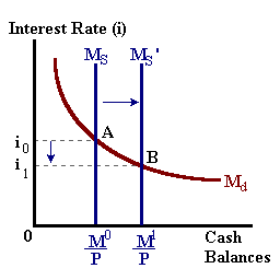
In the diagram below left, an increase in reserves is shown as an outward shift in the money supply line. As interest rates fall, the opportunity cost of holding cash balances also falls. The public will be willing to hold larger cash balances in the form of new deposits. In the diagram on the right we find that as interest rates fall, borrowing intended for investment expenditure increases thus shifting the AE line upwards. This is similar to an autonomous spending shock [note: in the diagram below-right, Z = A_o - h(r)] such that the increase in investment spending, working through the spending multipler will lead to an increase in income closer to the potential of the economy at Y₁:

Reserves ↑, → Excess Supply of Money, → > i ↓, M_d ↑,

i ↓ , r ↓, [A_o - h(r)] ↑ → I ↓, and Δ_[+]Y = α[A_o - h(Δ_[-]r)].

With an increase in the money stock...	Investment expenditure increases

10.3.3 Contractionary Monetary Policy

In the case of contractionary monetary policy, the Federal Reserve is reacting to inflationary pressure in the economy due to an increase in aggregate demand (more purchasing power) or a reduction in potential output perhaps due to an adverse productivity shock or an increase in factor prices. In both cases, the economy's ability to spend exceeds its ability to produce leading to upward pressure on output prices.

External Shock: an Increase in Aggregate Demand
(putting upward pressure on the Price Level)

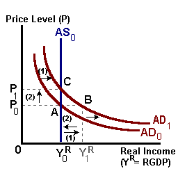
The diagram above models a demand-side shock pushing aggregate demand outwards (1). This creates an excess demand for goods -- demand greater that the potential of the economy to produce goods and services. The result is an increase in the price level (2). Left unchecked, rising prices will reduce purchasing power shown as a movement up AD. The net result is a higher price level (inflation) with no change in output.

The Fed will combat this increase in demand-side spending through a monetary contraction, pulling reserves out of the banking system, pushing interest rates upward and increasing the costs of borrowing to weaken investment spending and thus shifting aggregate demand back closer to its original level.

Reserves ↓,→ Excess Demand for Money, → i ↑, M_d ↓,

as

i ; r ↓, [A_o - h(r)] ↑ →; I ↓, and Δ_[-]Y = α[A_o - h(Δ_[+]r)].

The open market sale of government securities (the Fed selling bonds in exchange for reserves) would create a surplus of these securities in secondary bond markets thus driving their price down and yields up (Ψ ↑).

In reality the directive to the N.Y. trading desk from the Federal Open Market Committee will be to buy and sell securities until a particular interest rate (Federal Funds target) has been met. Because of day to day changes in the money multiplier, withdrawal and deposit activity, and other forces; the actual Federal Funds rate will hover around this target. However, if the goal of the Fed is to increase this short-term rate, other interest rates (i.e., the Prime Lending Rate) are likely to follow with the consequent effect on Investment expenditure decisions and ultimately Real GDP.

It is important to note that the Federal Reserve and monetary policy only affects short-term, low-risk rates. Usually the term and risk structure of all interest rates will follow. But with changes in inflationary expectations, investment opportunities, savings behavior, and uncertainty about the future other interest rates in the economy can rise or fall independent of actions by the Fed. It is the buying and selling in private financial markets that determine the full structure of interest rates which act as a barometer of the economy.