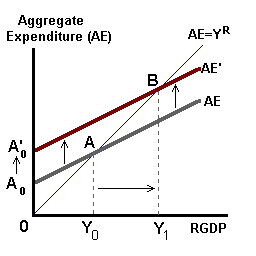
Our discussion of Fiscal policies will only include expansionary policies. As stated previously, contractionary policies tend to be politically unpalatable and thus seldom used for economic policy purposes. the expenditure line becomes steeper,Expansionary policies, therefore, include increased government expenditure, lower taxes (tax rates or redefinition of the taxable base) or both. Typically such policies would be used in cases where the economy is operating well below its potential. In such cases we would expect that there are excess resources available for production and thus little pressure exacted on the price level by these policies.
Discussion or evaluation of contractionary fiscal policy would just be the mirror image of what follows below.
The use of expansionary fiscal policy was first articulated by John Maynard Keynes in his General Theory of Employment, Interest, and Money (1936). This work, written in reaction to the events of the Great Depression, suggested that governments could stimulate effective demand for goods, where that demand was lacking in the private sector. He stated that the government could take bank-notes, put them in bottles and bury the bottles around the country. Individuals would go to some effort to dig up these bottles, acquire the bank-notes and spend some if not all of this newly-discovered purchasing power. This would create new demand for goods and services resulting in business firms increasing production levels and hiring additional workers.
To be more practical in his suggestion, Keynes, stated that governments could in a similar fashion, stimulate demand by increased public spending
(Δ[+]G)
on necessary public projects (administrative buildings, roads, dams, and other infrastructure) thus putting the unemployed to work in "gainful industry". These workers earning a legitimate income would then begin to spend on goods and services - spending that would lead to inventory depletions and thus create additional employment in the production and replenishment of these inventories.
Consumption expenditure is given by:
C = C0 + b(1 - t)Y
where 'C0 represents autonomous expenditure, 'b' is the MPC and 't' is the Tax rate. Consumption is proportional to income.
The other expenditure categories are simple autonomous expenditure:
I = I0, G = G0, NX = Xo - Mo
where: 'I'0' is autonomous investment spending, 'G'0' is autonomous government spending, 'X'0' is autonomous export spending and 'M0 represents autonomous import spending.
Summing the expenditure categories and solving for 'Y':
Y = C + I + G + NXor
Y = A0 + b(1-t)Y
given: A0 = C0+ I0+ G0 + X0 - M0
Y [1 - b(1-t)] = A0
The spending multiplier α may be written as:
α' = 1/[1 - b(1 - t)]
and
Ye = α '[Ao]
From this model, we can write:
Δ[+]G = Δ[+] Ao
or
Δ[+]YR = α[Δ[+] Ao]
Suppose that the economy was in equilibrium at some level (Y0) below full employment GDP (Y1) as shown by point A in the diagram below. A policy response in the form of an increase in government expenditure -- spending on privately- produced goods and services or public projects, would be modelled as an increase in autonomous expenditure (A0 → A1).

Business firms producing these goods or workers hired to work in public projects would receive this expenditure as new income and then spend part of this income on other goods and services. Throughout the economy other businesses and workers see a boost in income and also increase their spending -- the multiplier process. Real GDP (holding prices constant) would increase ((Y0 → Y1) by some multiple 'α' of the initial change in autonomous expenditure.
A reduction in taxes will have a similar effect on RGDP except, in this case, the change will occur through changes in disposable income and consequently on consumption expenditure.
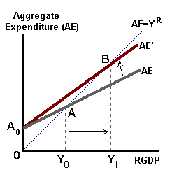
Lower tax rates increase the value of the spending multiplier 'α'. Given that this multiplier is defined as:
α = 1 / [1 - mpc(1 - t)],
as:
t ↓ , (1 - t) ↑,
therefore:
mpc(1 - t) ↑, -- the expenditure line becomes steeper as shown in the diagram above,
and as:
[1 - mpc(1 - t)] ↓, → α ↑
So:
Δ[-]t = Δ[+] α → Δ[+]YR = [Δ[+]α]Ao
It is important to note that in both of these examples, we are assuming no change in the aggregate price level. In reality, a fiscal expansion could put upward pressure on this price level which might mitigate some or all of the increase in real GDP.
If we focus on the real economy (Real GDP and corresponding expenditure categories) we might conclude that expansionary fiscal policy will be effective in increasing Real GDP. However, by taking into consideration the feedback role of financial markets, this may not always be the case.
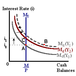
We know that the demand for money (cash balances) is affected by changes in aggregate income -- the transactions demand for money. Expansionary fiscal policy will lead to increases in aggregate income as s shown by the movement from points 'A' to 'B' in the diagram below-right. However these changes in income will also shift the demand for money 'Md' outwards -- more money being desired to facilitate increased spending. Holding the money supply 'MS' constant will result in an excess demand for cash balances. Individuals will make portfolio adjustments (selling financial assets in exchange for cash) pushing asset prices down and asset yields (and interest rates) up. In place of these portfolio adjustments, individuals may also attempt to borrow more from financial intermediaries (banks) but be unable to do so given the unchanging reserve position of the banking system.
| The Money Market | Crowding Out of Investment |
 |
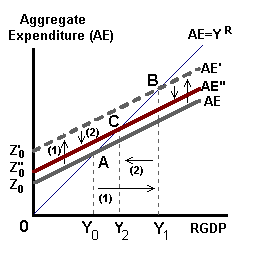 |
Interest rates will be pushed upwards given this excess demand. Higher interest rates will lead to higher borrowing costs resulting in some planned investment projects being abandoned (projects that are no longer profitable at these higher borrowing rates). As span class = "definition"investment expenditure declines, aggregate expenditure 'AE' also declines as shown by the movement from points 'B' to 'C' in the diagram below-right. In summary, because of activity in financial markets, the fiscal expansion has crowded-out private investment spending. This crowding out may be partial as shown below or could result in a dollar for dollar replacement of private spending by public spending.
|
|