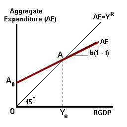
Certain expenditure decisions are affected by and assumed to be proportional to the level of income such that as aggregate income increases (Nominal GDP), expenditure increases by some fraction of this income change. We can think in terms of this expression representing an equilibrium condition (Ye) such that for one unique level of income, holding the price level constant, expenditure is exactly equal to that level of income:
Ye : Aggregate Income = Aggregate Expenditure
This conclusion of an equilibrium might be a rather strong assumption in a market economy where adjustment in prices result in an equilibrium within individual markets. As we aggregate accross markets, relative prices are not changing and any signals about the reallocation of resources are muted. Thus as a first step, we examine adjustments to an equilibrium condition through changes in production decisions, hiring, incomes earned and spending.
We begin developing our model with the notion that consumption expenditure 'C' is proportional to disposable income (gross income less taxes paid) with this proportional relationship being defined by the marginal propensity to consume 'b'. C0 represents autonomous consumption spending or consumption driving by other variables (i.e., changes in net-wealth, the price level or interest rates).
C = Co + b(Y - T), 0 < b < 1
Tax revenue 'T' is defined to be some fraction of income via the tax rate 't':
T = tY, 0 < t < 1
For algebraic simplicity we will define the other expenditure categories; investment 'Io', government 'Go', and net exports 'NXo' as being autonomous with respect to income (i.e., spending decisions independent of the level of national income). We will summarize this via a single variable 'Ao' known as autonomous expenditure:
Ao = Co + Io + Go + NXo
Thus, the expenditure equation can be written as:
[Y]income = [Co + b(Y-tY) + Io + Go + NXo]expenditure
or
Ye : [Y]income = [Ao+ b(1-t)Y]expenditure
as shown in the diagram below.
What is important here is that spending (expenditure) increase at some rate proportional to changes in income -- the income earned producing goods and services. This for every $1 increase in the level of output, spending increases by some amount less than $1.
(if: 0 ≤ 't' < 1, then 0 < '1 - t' ≤ 1 and if 0 < 'b' < 1, then 'b(1 - t)' < 1).
In this diagram, the 450 line represents a set of points where spending on goods and services is equal to the income earned producing those goods and services -- equilibrium between spending and income occurs on this line.

We can solve for 'Ye*', the equilibrium value of income as:
Y = Ao + b(Y - tY)
or
Y - b(1 - t)Y = Ao
or
Ye* = α [Ao],
where 'α' = 1 / [1 - b(1 - t)] and represents, what is commonly known as, the simple spending multiplier discussed below. For values of b less than one and t less than one, the value of the multiplier will be greater than one.
If the level of income is less than equilibrium, that is, a smaller level of production of goods and services; then spending will exceed this value and an unplanned depletion of inventories will occur. Business firms will react by hiring more workers and increasing the level of production. These workers will spend their increased income at some rate less than $1:$1 as discussed above. Production of goods and services increases at a rate greater than spending, inventories are replenished and the process continues until these inventories are completely restored -- equilibrium!
If, on the other hand, the level of income is greater than equilibrium, then spending is less than the rate of production and we have an unplanned accumulation of inventories. Business firms layoff workers, reduce the rate of production until theses excess inventories are eliminated. Again, spending falls by some amount less than $1:$1 until equilibrium is restored.
The key point of this story is that shocks to spending can lead to depletions or accumulations of inventories and an adjustment process will occur to determine a new equilibrium value.
Any time new spending is introduced into the economy (or if spending is removed), it will cause GDP (and other measures of national income) to change by some multiple of that spending shock. This takes place through the multiplier process in aggregate spending largely via changes in consumption expenditure.
For example, suppose that the marginal propensity to spend (changes in spending induced by changes in income) is equal to 0.50 [an MPC equal to 75% and tax rate of 1/3 -- 0.75 x (1 - 0.333) = 0.50]
Expenditure = Ao + 0.75(Y - 0.333Y)
=Ao + 0.50Y
Given our equilibrium condition: Y = AE (Aggregate Expenditure)
Y = Ao + 0.50Y
Since [1-b(1-t)] is less than 1, the spending multiplier 'α' will be greater than one such that:
Ye = 2.0[Ao]
and
Δ Ye = 2.0[Δ Ao]
An initial change in autonomous spending (for example, a shock in the form of an increase in government spending) of $20 (billion) is received as income by some person or business in the aggregate economy. This spending translates into an increase in income for that person who, given the propensity to spend, will increase his expenditure by $10 . This $10 in additional spending is received by someone else as income who spends 50% of that amount.
The spending flows through the aggregate economy such that when we total up all of the increases in income we find that aggregate income has increased by $40 billion -- 2.0 times the initial spending shock. This is known as the multiplier process.
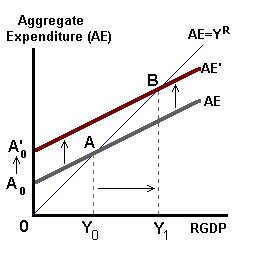
Changes in autonomous expenditure (changes in Investment, Government spending, or Net exports for example) will shift this line up or down. Working through the multiplier, the equilibrium level of aggregate income increases by some multiple of this autonomous change.

Changes in interest rates may affect both autonomous consumption and autonomous investment. Changes in the tax rate will affect the value of the multiplier such that:
as t ↑ , α ↓.
Changes in exchange rates affects both exports and imports -- for example, a stronger dollar will reduce exports, increase imports and cause NX to fall.
|
|