Douglas A. Ruby
Revised: 01/18/2003
Price Level Determination
Macroeconomic Theory
Employment, and Prices
Long Run Aggregate Supply
Aggregate Supply represents the ability of an economy to produce goods and services. In the Long Run this ability to produce is based on the level of production technology and the availability of factor inputs. As stated earlier, production refers to the conversion of inputs -- the factors of production into desired output. A production function is often written as follows:
Y*t = f(Lt,Kt,Mt )
where Y* is an aggregate measure of potential output in a given economy.
- L represents the quantity and ability of labor input available to the production process.
- K represents capital, machinery, transportation equipment, and infrastructure.
- M represents the availability of natural resources and materials for production
Over time with growth in the availability of factor inputs or technological improvement, the level of potential output increases. Thus in the Long Run we define the Aggregate Supply (ASLR) function as being influenced by those elements included in the production function and independent of the price level.
| figure 1 -- Aggregate Production | figure 2 -- Aggregate Supply |
 |  |
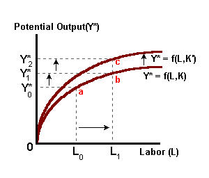
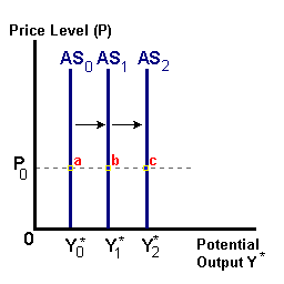
In the above diagrams we find that in time period '0' the economy is capable of producing a level of output equal to Y*0 (point a). Growth in the amount of labor ('a' to 'b') available allows for the production of more output with existing levels of technology (Y*0 to Y*1). More capital (or materials) or improvements in productivity will lead to an even greater potential to produce (Y*1 to Y*2) at each-and-every price level (i.e., 'b' to 'c').
Changes in the Price LevelIn the aggregate economy the price level is determined by the balance (or imbalance) between the ability to produce goods and services and the ability to spend to acquire those same goods. The ability to produce is summarized by the long run Aggregate Supply (AS) function based on the level of technology and availability of factor inputs. The ability to spend is summarized by the Aggregate Demand (AD) relationship which represents combinations of income and interest rates such that product markets and financial markets are in equilibrium. As prices rise, purchasing power falls, and thus the quantity of goods and services that can be acquired with a given nominal income declines. Aggregate Demand represents this inverse relationship between the price level and purchasing power.

A supply-side shock, such as an increase in labor productivity, would shift AS outward -- there is a greater potential to produce at each and every price level. We can see this change in figure 1 to the left. This shock, in time, creates an excess supply of goods (Y* > YR) and puts downward pressure on the price level. As prices fall, purchasing power increase reflecting an increase in the ability to spend (i.e., a movement from A to B). The net result in an increase in output and spending and a lower price level.

In figure 2 to the left, we have a demand-side shock perhaps the result of an increase in government spending. This shock shifts the AD relation outward. Initially there is an excess demand for goods (A to B) evidenced by a depletion of inventories. Given that potential output has not changed, in time this excess demand will cause the price level to increase . As prices increase, purchasing power falls and the ability to spend decreases (B to C). The net result of this shock is an increase in the price level with no change in output or real spending.
Price Expectations and Aggregate Supply in the Short Run
A different approach to understanding aggregate supply is in the form of the Lucas Aggregate Supply equation. This equation is derived from individual supply equations (over 'n' goods) for different economic agents based on actual prices and expected prices:
Yit = Y*t + b(Pit - E[Pit]) -- for i = 1 ... n goods.
Expectations about the agent's own price are derived by that agent based on observations about the general price level: E[Pit] = f( Pt ). If the firm's actual price 'Pit' exceeds the expected price value E[Pit] then this is situation is characterized by the agent as an increase in the relative price for the agent's product or services (the agent perceives that the market is placing a higher value on its product) and thus this agent will devote more resources to production such that Yit > Y*0 where Y* represents some normal level of output by that agent.
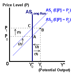
Aggregating over all agents in the economy, we have the aggregate supply function which states that actual output will exceed the normal level of output (Y1 > Y*0 in the diagram below) when the actual price level exceeds the expected price level (P1 > P0) perhaps due to some unanticipated shock to the economy or monetary system. An equation for short-run Aggregate Supply (AS) can be defined as:
and shown in the diagram below:Yt = Y*0 + β(Pt - E[Pt])
| figure 3 -- Lucas Aggregate Supply |
 |
In time these economic agents will discover that the price of their particular good has not changed relative to the price of other goods in the economy. These agents will discover that they have made incorrect production decisions (i.e., overproduced) and make the necessary corrections. This involves an upward revision of their price expectations (Pt = E[Pt]) and a reduction in output (B to C in the above diagram). Even though output temporarily exceeded the potential of the economy, in the long run the level of output will return to this potential level (Yt = Y*0).
In summary, the only way a change in the price level can affect supply (production) decisions in an aggregate economy is if the price level 'P' exceeds that expected 'E[P]' by individual producers. Ultimately changes in (potential) output are the result of changes in the available of resources or productivity (and technology).
Concepts for Review:
- Aggregate Demand
- Aggregate Supply
- Excess Demand for Goods
- Excess Supply of Goods
- Inflation
- Product Markets
- Price Level
 |
 |
 |