Original Position An Increase in Labor Input An Increase in Capital Input
Production refers to the conversion of inputs, the factors of production, into desired output. A production function for a particular good or service is often written as follows:
Xi = f (L,K,M,R)
where Xi is the quantity produced of a particular good or service and:
A positive relationship exists among these inputs and the output such that greater availability of any of these factors will lead to a greater potential for producing output. In addition, all factors are assumed to be essential for production to take place. The functional relationship f(.) represents a certain level of technology and know how, that presently exists, for conversion these inputs into output such that any technological improvements can also lead to the production of greater levels of output.
In order to better understand the technological nature of production, we distinguish between short run production relationships where only one factor input may vary (typically labor) in quantity holding the other factors of production constant (i.e., capital and/or materials) and the long run where all factors of production may vary. The short run allows for the development of a simple two variable model to understand the behavior between a single variable input and the corresponding level of output. Thus we can write:
Xi = f(L;K,M,R)
or
Xi = f(L)
For example we could develop a short run model for agricultural production where the output is measures as kilograms of grain and labor is the variable input. The fixed factors of production include the following:
We might hypothesize the production relationship to be as follows:
| Input (L) |
Output (Xgrain) |
MPL |
| 0 | 0 kg | - |
| 1 | 100 | 100 |
| 2 | 200 | 100 |
| 3 | 300 | 100 |
| : | : | 100 |
| 10 | 1,000 | 100 |
In this example we find that each time we add one more unit of labor, output increases by 100 kg. The third column MPL defines this relationship. This column measures the marginal productivity of labor -- a measure of the contribution of each additional unit of labor input to the level of output. In this case, we have a situation of constant marginal productivity which is unrealistic with production in the short run. Constant marginal productivity implies that as labor input increases, output always increases without bound -- a situation difficult to imagine with limited capital and one acre of land.
A more realistic situation would be that of diminishing marginal productivity where increasing quantities of a single input lead to less and less additional output. This property is just an acknowledgment that it is impossible to produce an infinite level of output when some factors of production (machines or land) fixed in quantity. Numerically, we can model diminishing marginal productivity as follows:
| Input (L) |
Output (Xgrain) |
MPL |
| 0 | 0 kg | - |
| 1 | 100 | 100 |
| 2 | 180 | 80 |
| 3 | 240 | 60 |
| 4 | 280 | 40 |
| 5 | 300 | 20 |
| 6 | 300 | 0 |
In this case, additional labor input results in additional output. However, the contribution of each additional unit of labor is less than previous units such that the sixth unit of labor contributes nothing to output. With 5 or 6 workers, the available amount of land cannot support additional output.
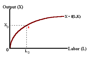
A short run production relationship can be modeled in the diagram below. In this example, labor is the variable factor input and land, capital, and entrepreneurship are fixed in quantity. There is a positive relationship between labor input and output levels, however, as additional labor in used, less and less additional output is produced (click on the second button). The shape of this production function is consistent with the law of diminishing marginal productivity.

Changes in the amount of capital or other fixed factors or in the level of technology will lead to an upward shift in the production function (click on the third button) such that a greater level of output may be produced with the same amount of labor input.
If we extend our model of production to two (or several) goods, we can develop a more realistic notion of production relationships. In a world of scarce resources, business firms producing different goods are competing for the same pool of factor inputs. In the short run labor is available for the production of one or a combination of goods. However, the desire to increase production of one good 'X' will come at the expense of another good 'Y' as labor or other resources are relallocated from the first good to the second.
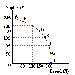
In the table below, we can model this competition for resources between two goods: Apples and Bread. In this example, an additional unit of labor directed to bread production allows for producing 25 additional units of bread (the marginal productivity of labor in bread production is constant). Separately, additional units of labor applied to apple production allows forthe producing anywhere from 0 to 185 units of apples.
Pt. |
X (Bread) |
MPL,Bread | Pt. |
Y (Apples) |
MPL,Apples |
| A | 0 | - | H | 0 | - |
| B | 60 | 60 | G | 50 | 50 |
| C | 110 | 50 | F | 95 | 45 |
| D | 150 | 40 | E | 135 | 40 |
| E | 180 | 30 | D | 170 | 35 |
| F | 200 | 20 | C | 200 | 30 |
| G | 210 | 10 | B | 225 | 25 |
| H | 215 | 5 | A | 245 | 20 |
Working with an assumption that the amount of labor input is fixed in supply at 8 units, this labor must be shared between bread and apple production. If we happen to be producing 245 units of apples (point A), then all 8 units of labor are being used for this purpose. The desire to produce bread requires a reallocation of labor from apple production to bread production. In the table above, we can show this as a movement from point A to point B. We are able to produce 60 units of bread (0-60 units) but at the expense producing 20 apples (245 - 225 bushels). These 20 bushels of apples represent the opportunity cost of bread production (i.e., each unit of bread "costs" 60/20 = 3 bushels of apples. If we move from point B to point C, the additional 50 loaves of bread (60 - 110), come at the expense of 25 bushles of apples (225 - 200 bu). Because of diminishing marginal productivity in apple production, the production of 50 additional units of bread requires that more and more apples are given up -- one loaf of bread costs 2 bu of apples.. Stated differently, we can say that the opportunity cost of producing bread is increasing.
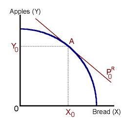
The diagram below summarizes the numbers in the above table. Points on the blue curve -- the Production Possibilities Frontier represent an efficient use of resources. Points within the curve represent an inefficient use of resources -- resources and technology allow for producing more Apples, Bread, or more of both. Movement along the curve imply that a tradeoff exists in production when resources are scarce or fixed in supply. Finally points (combinations of the two goods) beyond the frontier are unattainable with existing levels of technology and resource availability.

The slope of the PPF is known as the Marginal Rate of Transformation (MRT), and is calculated as the the ratio of marginal productivities.
Specifically:
MRT = MPy /MPx = Marginal Costx /Marginal Costy
given that: Marginal Costi = wage rate /MPi
This ratio measures the opportunity cost of using resources in producing one good in terms of the alternative use of those resources used in the production of other goods. Given the role of diminishing marginal productivity; as resources are allocated away from good Y towards good X, the opportunity cost (|MRT|), of producing more of good X, increases.
If resources were to be allocated in the opposite direction, the same would be true -- the opportunity cost of producing more of good Y would also increase in terms of foregone production of good X.
Suppose that we are producing at point D in the above diagrams. If we transfer one unit of labor away from apple production to bread production, we must give up 35 units of apples and gain 30 units of bread. Thus the opportunity cost of each loaf of bread is 7/6 (1.17) bushels of apples. Bringing relative prices into the picture, we might find that the price of apples 'Papples' is $2.00 and the price of bread 'Pbread is $3.00.
Or,
PR = [Px / PY] = [Pbread / Papples] = 1.50.
Stated differently, (as a Terms of Trade), we find that we are willing to trade 1 unit of bread for $3.00 and with that $3.00, we could then acquire 1.5 units of apples. One unit of bread is worth 1.5 units of apples given these prices.
If we compare the relative price of bread to the opportunity cost of bread, we find that the value of bread in terms of apples is greater than the opportunity cost of producing bread:
Pbread / Papples > MRT
From a social point of view, we should be allocating more resources towards bread production and away from apple production. With the reallocation of resources, the opportunity cost of bread production will rise. This reallocation should continue until the following is true:
PR = MRT
or
Pbread / Papples = MCbread / MCapples

If the price of bread were to fall, say to $2.00 per unit (click on the Next button), then the relative price of bread would be equal to 1.0 (i.e., each unit of bread is exactly equal to the value of one unit of apples) and PR ↓. With this change, the value of bread, in terms of apples, is less than the opportunity costs of producing bread. In this case we should allocate resources away from bread production (click on the Next button again). This reallocation will cause the opportunity cost of bread to fall until it is just equal to the prevailing relative price. (Click on the Next button again to repeat.)
|
|