Models of labor supply begin with the assumption that workers choose combinations of hours-worked and income towards the goal of maximizing their level of utility given the time constraint of the number of hours in the day.

In most labor supply models, work is considered to be an undesirable good. Hours not worked are called leisure hours with leisure time being the desirable good. The problem of the worker appears as follows:

maximize U = f(Income, Leisure)
s.t.
labor hours + leisure hours < 16 waking hours.

The above expression may be read as "maximize utility (satisfaction) which is a function of income and leisure hours (both desirable goods) subject to the number of waking hours available in a day". The above model may be expressed in terms of labor hours 'L' as follows:

max U = f(w L, 16-L),

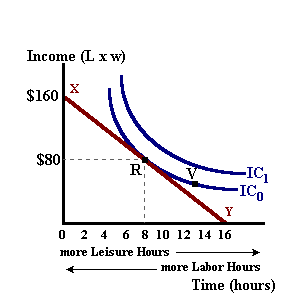
where 'w' is the prevailing wage rate. In order to understand the above model, we will use indifference curve analysis to examine the effects of a changing wage rate on the number of labor hours supplied. In figure 1, any point on the curve IC_o, which represents a combination of income and leisure hours, will give the individual the same level of satisfaction. The individual would be indifferent between point ' R' and point 'V' on this curve.

figure 1 -- A worker optimum

Points on the curve IC₁ represents combinations (or bundles) of income and leisure that give the individual a higher level of satisfaction. The line 'XY' represents the budget constraint imposed by the number of waking hours available in a day (note: the horizontal intercept is equal to 16) with a slope determined by the class = "definition"real wage rate 'w'¹.

In any indifference curve model, equilibrium for the individual exists where an indifference curve is just tangent to the budget line. In the diagram above this occurs at point 'R'. The economic interpretation of this tangency is that this is the point where the marginal rate ofsubstitution 'MRS'² between income and leisure time is just equal to the price of leisure time as measured by the real wage rate. This real wage represents the opportunity cost of leisure time in terms of foregone income.

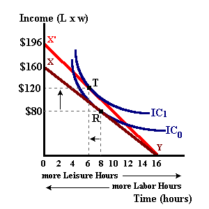
An increase in the real wage rate will serve to rotate the budget line upwards (holding the horizontal intercept constant) and allow for a tangency with the higher indifference curve as shown in figure 2. As wages rise, the worker is better off with the ability to earn more with each hour of work or to maintain current income levels with less work (and thus the ability to consume more leisure time).

figure 2a -- An increase in wages (strong substitution effect)	figure 2b -- Corresponding Labor Supply Curve

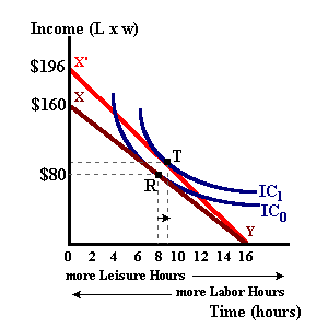
In figure 2a, an increase in the wage rate from $10 per hour to $12 per hour had the effect of increasing the equilibrium level of income and decreasing the number of leisure hours (work hours increased) as indicated by the solid curve IC₁. In this case the worker reduces the amount of leisure time from 8 hours to 6 hours.It could have been the case that the new equilibrium point was defined by the curve IC₁' in figure 3. In this case the worker reduced the number of work hours upon receiving the wage increase. Both cases are theoretically possible due to the relative size of the income and substitution effects. The total change in leisure hours is called the total effect which is the summation of income and substitution effects. With a wage increase, leisure time becomes relatively more expensive (in terms of foregone wages) so the worker will substitute away from leisure time -- the substitution effect is negative for a wage increase.

figure 3a -- An increase in wages (strong income effect)	figure 3b -- Corresponding Labor Supply Curve

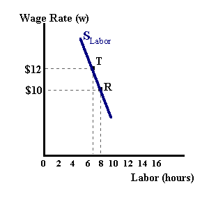Additionally, as income rises with the wage increase individuals will want to consume more leisure assuming that this good is a normal good -- the income effect for a wage increase is always positive. If the positive income effect is less than the negative substitution effect, the total effect will be negative and the worker will consume less leisureand more work. This will lead to a "normal" upward sloping labor supply curve (the relationship between the real wage and labor hours supplied). If the income effect is greater than the substitution effect, the worker will consume more leisure (a positive total effect) and less work. In this case the labor supply curve will be "backward-bending" or represent an inverse relationship between the wage rate and labor hours supplied (see figure 3).

Empirical studies have concluded that, when we aggregate among all workers, the labor supply curve is upward sloping and fairly steep (that is, labor supply decisions are highly wage inelastic or insensitive to changes in the wage rate). Stronger influences on labor supply come about with changes in population, labor force participation rates (demographic changes) and immigration flows.

Labor Demand and Market Equilibrium

If we assume that labor supply is positively related to the real wage:

L_s = f_[+](w)

then any increase in labor demand 'L_d' will lead to higher equilibrium quantities of labor being made available to labor markets at higher real wages. However, before we discuss equilibrium conditions, we need to take a look at the determinants of labor demand.

The demand for labor results from producers seeking labor input as one of several factor inputs into the production process: X = f(L,K,M).

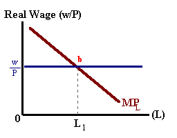
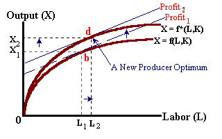
Referring back to a producer optimum, we find that the profit maximizing firm will hire labor up to the point where the marginal productivity of the last worker hired 'MP_L' is just equal to the real wage 'w/P_x'. This is shown graphically in the diagram below left by the tangency between the production function (slope = MP_L) and the dotted iso-profit line (slope = w/P_x) or in the diagram below right by the intersection of MP_L and w/P as defined by point ' b':

figure 4 -- The Profit Maximizing Quantity of Labor Input

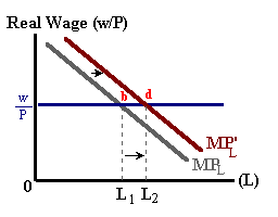
Changes in labor productivity, either due to technological improvement or by the addition of more capital per worker will lead to an upward shift in the production function (more output for each unit of labor input) and an outward shift in MP_L (each worker is more productive at the margin). Holding the real wage constant will result in more labor being hired and more output being produced as shown in the diagrams below:

figure 5 -- An Increase in Labor Productivity

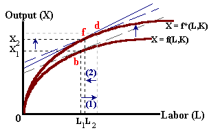
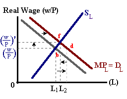
In reality, this type of shock when matched with an upward sloping labor supply curve should lead to an increase in the real wage. This higher real wage is necessary to induce more workers into the labor market or to induce existing workers to work longer hours (in both cases sacrificing leisure time). This is shown below in figure 6. The increase in productivity shifts the production function upwards and the marginal product of labor outwards (b → d). However, this excess demand for labor leads to an increase in nominal and real wages leading to an upward movement along the new labor demand curve in the right diagram and a counter-clockwise rotation in the iso-profit line in the left diagram (d → f).

Thus a complete model of this type of shock (an increase in productivity) will lead to a larger equilibrium quantity of labor (L₁ → L₂) and higher real wages.

figure 6 -- An Increase in Labor Productivity

Other types of shocks that may affect labor markets would be in labor supply either due to changes in labor force participation rates or changes in immigration patterns. For example, a relaxation of immigration policies (i.e., the H-visa program of the late 1990's in support of the "tech" boom) would shift labor supply outwards putting downward pressure on the real wage. This decline in real labor costs might lead business firms to hire more labor, increasing the level of production and increasing the output of the economy.