Rational Expectations is the notion that households, business firms and other economic agents use all available economic information in their decision making. These agents remember past events, outcomes and consequences of past policy actions. This memory keeps them from being tricked by tweaks or shocks to the price level or other nominal magnitudes. Instead they will quickly update their expectations about future real economic activity

The Rational Expectations Model can be summarized through the use of four equations to define economic activity:

1. The Aggregate Demand Equation:

AD = (C + I + G + NX) = P_tY_t^R

or

M_tV = P_tY_t^R

Where M_tV represents total expenditure as defined by the product of the money stock and its velocity (the number of times a unit of currency is used for subsequent transactions). This expression can be rearranged as:

P_t = (V/ Y_t^R)M_t

2. The second equation represents a money supply rule which states that the money supply is proportional to the level of real economic activity 'Y^R' with the addition of a random error term allowing for unexpected monetary shocks to the system:

M_t = ΘY^R_t-1 + ε_t

Over time these shocks tend to cancel out such that E[ε_t ] = 0.

3. The third equation is the Lucas Aggregate Supply equation. This equation is derived from individual supply equations for different economic agents based on actual prices and expected prices:

Yⁱ_t = Y^*_t + b(Pⁱ_t - E[Pⁱ_t])

Expectations about the agent's (business firm's) own price are derived by that agent based on observations about the general price level: E[Pⁱ_t] = f( P_t ). If the firm's actual price 'Pⁱ_t' exceeds the expected price value E[Pⁱ_t] then this is situation is characterized by the agent as an increase in the relative price for the agent's product or services (the agent perceives that the market is placing a higher value on its product) and thus this agent will devote more resources to production such that Yⁱ_t ã Y^*_t where Y* represents some normal level of output by that agent.

Aggregating over all business firms in the economy, we have the aggregate supply function which states that actual output will exceed the normal level of output when the actual price level exceeds the expected price level perhaps due to some unanticipated shock to the economy or monetary system:

Y_t = Y*_t + β(P_t - E[P_t]

4. Finally, we have a fourth equation defining price expectations as being rational that is: that expectations about the general price level are based on all available information in the most recent time period I_t-1

E[P_t] = E[P_t | I_t-1]

This available information sometimes known as the Information Set may include items such as growth rate in the money stock, fiscal policy changes, factor price shocks, and existing inflationary expectations among others.

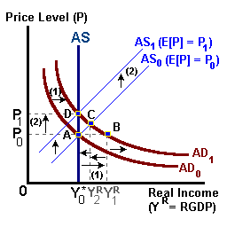
The model works as follows (refer to the figure below):

• Given an unanticipated increase in the money supply resulting in the shock term being positive (Ε_t > 0), aggregate demand will shift outward as defined in traditional demand-side models (A to B below).
• This increase in demand-side spending will put upward pressure on the general price level and the shift in demand leads to a movement along the upward aggregate supply schedule. (A to C). As prices increase, purchasing power declines (B to C).
• This increase in the price level is interpreted by different economic agents as an increase in the relative price for their product or service. These agents respond by increasing their level of output. As time passes, these economic agents find that the price increase represented an increase in the absolute price level rather than an increase in relative prices. They adjust their price expectations accordingly as shown by an inward shift in aggregate supply (AS₀ to AS₁). Output declines, prices increase and purchasing power is further reduced. (C to D).

Rational Expectations Model

These agents were tricked into producing more output such that they find that they have overproduced. The response to this information about the absolute price level leads to an updating in the agents' expectation about general prices (i.e., E[Pⁱ_t] are adjusted upwards). Given this update in price expectations, the aggregate supply function shifts upwards such that over time the actual level of output Y* remains unchanged.

However, the general price level has increased. Although in the above discussion, the demand-side shock was an unanticipated increase in the money stock, similar results would occur from changes in autonomous expenditure resulting from any type of expansionary fiscal policy--the outward demand-side shift leads to a temporary increase in output until price expectations are updated resulting in an upward shift in aggregate supply.