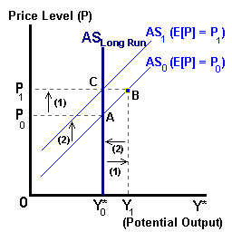
In the last section, we examined changes in the price level and inflation as a result of imbalances between potential output and Real GDP -- the output gap. A different approach is to examine changes in output (or production decisions) in reaction to a mismatch between the price level and expectations about that price level.
This different approach to understanding aggregate supply is in the form of the Lucas Aggregate Supply equation. This equation is derived from individual supply equations (over 'n' goods) for different economic agents based on actual prices and expected prices:
Yit = Y*t + b(Pit - E[Pit]) -- for i = 1 ... n goods.
Expectations about the agent's own price are derived by that agent based on observations about the general price level: E[Pit] = f( Pt ). If the firm's actual price 'Pit' exceeds the expected price value E[Pit] then this is situation is characterized by the agent as an increase in the relative price for the agent's product or services (the agent perceives that the market is placing a higher value on its product) and thus this agent will devote more resources to production such that Yit > Y*0 where Y* represents some normal level of output by that agent.
Aggregating over all agents in the economy, we have the aggregate supply function which states that actual output will exceed the normal level of output (Y1 > Y*0 in the diagram below) when the actual price level exceeds the expected price level (P1 > P0) perhaps due to some unanticipated shock to the economy or monetary system. An equation for short-run Aggregate Supply (AS) can be defined as:
Yt = Y*0 + β (Pt - E[Pt])
and shown in the diagram below:

In time these economic agents will discover that the price of their particular good has not changed relative to the price of other goods in the economy. These agents will discover that they have made incorrect production decisions (i.e., overproduced) and make the necessary corrections. This involves an upward revision of their price expectations (Pt = E[Pt]) and a reduction in output (B to C in the above diagram). Even though output temporarily exceeded the potential of the economy, in the long run the level of output will return to this potential level (Yt = Y*0).
In summary, the only way a change in the price level can affect supply (production) decisions in an aggregate economy is if the price level 'P' exceeds that expected 'E[P]' by individual producers. Ultimately changes in (potential) output are the result of changes in the available of resources or productivity (and technology).
The Adaptive Expectations model is based on the notion that economic agents develop forecasts of future inflation based on past actual rates adjusted for their own past expectations. Specifically, inflationary expectations are calculated by using a weighted average of past actual 'πt' and past expected inflation 'E[π t-1]':
E[πt] = Θ πt-1 + (1- Θ)E[πt-1] where 0 < Θ < 1
By algebraically rearranging this equation we have:
E[πt] = E[πt-1] + Θ{πt-1 - E[πt-1]}
where the term in the brackets represents the forecast error made by the economic agent in attempts to determine the previous rate of inflation. From this second equation current inflationary expectations are defined to be the sum of the rate previously expected and this forecast error. The rate by which economic agents adapt to accelerating inflation depends on the value of the weight 'Θ' assigned to past expected inflation in developing current inflationary expectations. Note if this weight is equal to one then current inflationary expectations are exactly equal to the size of this forecast error.
| (Θ = 0.10) | (Θ = 0.50) | ||
Time |
Actual Inflation |
Expected Inflation |
Expected Inflation |
| 1 | 5% | 3.2% | 4.0% |
| 2 | 5% | 3.4% | 4.5% |
| 3 | 5% | 3.6% | 4.8% |
| 4 | 8% | 4.0% | 6.4% |
| 5 | 8% | 4.4% | 7.2% |
| 6 | 8% | 4.8% | 7.6% |
| 7 | 8% | 5.1% | 7.8% |
| 8 | 8% | 5.4% | 7.9% |
| 9 | 8% | 5.7% | 8.0% |
| 10 | 8% | 5.9% | 8.0% |
In the above table, we see that in the absence of an acceleration of inflation the value of theta influences how quickly economic agents adjust to the shock in time period 4.
| (Θ = 0.10) | (Θ = 0.50) | ||
Time |
Actual Inflation |
Expected Inflation |
Expected Inflation |
| 1 | 5% | 3.2% | 4.0% |
| 2 | 6.5% | 3.5% | 5.3% |
| 3 | 8.0% | 4.0% | 6.7% |
| 4 | 12.5% | 4.9% | 9.6% |
| 5 | 14.0% | 5.8% | 11.8% |
| 6 | 15.5% | 6.8% | 13.7% |
| 7 | 17.0% | 7.8% | 15,4% |
| 8 | 18.5% | 8.9% | 16.9% |
| 9 | 20.0% | 10.0% | 18.5% |
| 10 | 21.5% | 11.2% | 20.0% |
In an environment of an acceleration of inflation, the agent's expectations will never quite catch up to the actual rate. For this reason, many models assume that the economic agent uses other relavent information such as growth rate in the money supply, the rate of unemployment, and measures of structural capacity utilization within the economy in developing inflationary expectations. These models are known as Rational Expectations models.