3.2.1 Production

Production refers to the conversion of inputs, the factors of production, into desired output. An economy-wide production function is often written as follows:

X^* = f(L,K,M)

where X* is an aggregate measure of goods and services produced (output) in a given economy.

• L represents the quantity and ability of labor input available to the production process.
• K represents capital, machinery, transportation equipment, and infrastructure.
• M represents the availability of natural resources and materials for production

A positive relationship exists among these inputs and the output such that greater availability of any of these factors will lead to a greater potential for producing output. The functional relationship f(.) represents a certain level of technology and know how that presently exists for conversion of these inputs into output such that any technological improvements can also lead to the production of greater levels of output.

In order to understand the creation of wealth and the engine for economic growth that will provide for increasing standards of living, we must first start with an understanding of several characteristics govern aggregate production relationships.

• First, is the law of diminishing marginal productivity. Holding other factors of production constant (i.e., capital and/or materials), increasing quantities of a single input lead to less and less additional output.
• Second, is that all factors are essential in production and to some degree one factor may be substituted for another factor of production. Increasing the amount of capital or machinery can replace some labor but not all of the labor in a production process. Increasing amounts of labor (greater care being taken in production to avoid waste) can reduce the need for some material inputs.
• Third is that, for production in the aggregate, there are constant returns to scale. This property refers of the ability to double output simply by doubling the quantity of all the available inputs. A simple way to understand this is based on the idea that any production process may be replicated. Thus if a certain quantity of grain is being produced on one acre of land with 5 units of labor input and 3 pieces of capital, then by replicating this production process the quantity of grain produced may be doubled.

3.2.2 The Cobb-Douglas Production Function

One specific mathematical relationship that possesses these three properties is the Cobb-Douglas production function. This particular representation is one of several possibilities and may be written as follows:

X_i = A_tL^αK^βM^γ

where L, K, M represent the factor inputs listed above, A represents a measure of technology at time period 't', and the exponents represent production parameters (actually output elasticities) for each factor input. The fact that it is multiplicative in the inputs reflects the notion that one factor may be substituted for another. Diminishing marginal productivity requires that the exponents α, β, and γ each take on values less than one. Each input being essential and making a positive contribution to output implies that these exponents be strictly greater than zero. Finally, constant returns to scale implies that α, β, and γ sum to one.

With increasing returns to scale these exponents will sum to a value greater than one and with decreasing returns to scale, these exponents sum to a value less than one.

Returns to scale represent one dimension of production technology in the long run. This concept governs how costs change as production levels are altered. Under constant returns to scale, a doubling of output results in an exact doubling of production costs. In the case of increasing returns, costs increase at a rate less than than change in output such that average (per-unit) costs decrease with increasing levels of output. On the other hand, under decreasing returns to scale, costs increase at a rate greater than production. In this case, increasing production levels are matched by increasing per-unit costs.

3.2.3 Profit Maximizing Behavior

We also need to examine the behavior of those involved in the production process. One assumption is that of profit-maximizing behavior in that economic agents attempt to maximize the difference between the revenue from the sale of a particular good or service and the costs of production. We can write the following:

max π = R-C

or

max π = P_xX - [wL + rK + zM]
s.t X = f(L,K,M).

The objective function can be rewritten by solving for the variable 'X' as follows:

X = [(π + FC)/P] + (w/P)L

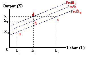
where FC represents the fixed costs of production (rK+nM). This expression is known as an iso-profit function with the term in the brackets being the intercept which represents a given level of profits and the term (w/P)-- also known as the real wage rate, represents the slope of this function. Any point on a particular line represents i given level of profits. For example, in the diagram below:

Iso-Profit Lines

The combination of L₀, X₀ corresponds to a level of profits of π₀. Likewise the combination of L₂ (greater costs) and X₂ (more revenue) also corresponds to this same level of profits (pi₀) -- revenue and costs increase by the same amount. However, the combination of L₁ and X₁ correspond to a greater level of profits relative to the combination of L₀, X₀ (revenue increases more than costs).

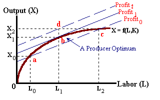
By adding the production function to the above diagram, we find that the input- output combinations as defined by points 'a', 'b', and 'c' are all within the limits of available technology. Point 'd' however, is unattainable -- a level of output of X₂ is impossible with a level of labor input of L₁.

A Producer Optimum

At point 'b', we find that we achieve the greatest level of profits possible with this existing level of technology. At this point the production function is just tangent to iso-profit line 'profit₁. This point is known as a producer optimum.

Mathematically, we can solve for this producer optimum by substitution of the constraint into the objective function,

max π = P_x[f(L,K,M)] - wL -rK - zM

and solving with respect to labor input we can derive the following:

δπ/δL = P_xMP_L - w = 0,

This result can be interpreted in a variety of ways.

• First we could write (using labor) P_xMP_L= w, where the left-hand side represents the marginal revenue product of labor -- that is the contribution of one more unit of labor input to the firm's revenue. The right-hand side 'w' represents the prevailing nominal wage rate or the cost of hiring that additional unit of labor. Profit maximization implies that the contribution to revenue (using monetary units of measure) is just equal to the contribution to costs in the hiring of one more unit of a factor input.
• Second, we can rearrange the terms and write MP_L = w/P_x. This expression states that profit maximization implies that the contribution of each additional unit of labor input to output must be paid a real wage (a measure of purchasing power) equivalent to that level of contribution.
• Third, we could write P_x = w/MP_L or P_x = MC which states that profit maximization occurs when the revenue from selling one more unit (marginal revenue) of a particular good 'P_x' is just equal to the cost of producing one more unit (marginal cost) of that good.

3.2.4 The Contribution of Factor Inputs to Economic Growth

From our look at national income accounting, we observe that for the U.S. economy (based on the income approach), that labor income historically has maked up roughly 70% of national income and non-labor income (proprietor's income, net rental income, corporate income, and net interest income) makes up the remaining 30% of national income. (We must note that, recently, labor's share of national income has fallen to roughly 62% -- something that must be kept in mind.)

Using the 70%/30% shares, we can be write:

NGDP = PX* = wL + rK,

wL = 0.70PX*, and
rK = 0.30PX*

Using the Cobb- Douglas production function with 'L' and 'K' representing labor input and non-labor input respectively and given constant returns to scale (,1 - α = β), we can write:

X* = AL^αK^{1 - α},

and

MP_L = α(X*/L) and MP_K = (1-α)(X*/K)

Note that the variable 'M' representing materials has been dropped under the assumption that labor and capital are combined in the extraction of these raw materials and the above factor payment percentages represents compensation for these types of activities.

With profit maximizing behavior in competitive markets:

P_xMP_L - w = 0

or

MP_L = w/P_x

and similarly

MP_K = r/P_x

Therefore

α(X*/L) = w/P

α = wL / PX* {labor's share of income}

(1 - α)(X*/K) = r/P

or

(1 - α) = rK / PX* {capital's share of income}

which implies that (roughly)

α = 0.70 and (1 - α) = 0.30

and

X^* = AL^0.70K^0.30

It can be shown that:

dX^* = [ΔX^*/ ΔA]dA + MP_LdL + MP_KdK

dX^* = [L^αK^(1-α)]dA + [α X^*/L]dL + [(1 - α)X^*/K]dK

and dividing through by 'X^*',we can write, noting that (L^αK^(1-α))/AL^αK^(1-α) = (1/A)]:

%Δ X^* = %ΔA + α[%Δ L] + (1 - α)[%Δ K]

Expressed differently, the rate of economic growth may be expressed as:

%ΔRGDP = %Δ X^* = %Δ A_t + 0.70[%Δ L] + 0.30[%Δ K]

Economic growth is thus the sum of the rate of growth in technology in addition to a weighted average of the rate of population growth and the rate in which capital accumulates. An interesting implication of this is that, holding other factors constant, a population growth rate of 1% leads to a less than one percent growth rate in output--a decline in the Standard of Living. In order to maintain or improve these Living Standards, there must be an accumulation of capital and/or technological progress.

Endnote: Between the end of WW II and the late 1990's, the rate of economic growth in the U.S. (%Δ RGDP = %ΔY*) has been in the neighborhood of 3.1% annually. During this time the labor and capital share of income was in the range of 70%, 30% respectively. Population growth and growth in the labor force (%ΔL) was somewhere around 1.2% per year. Thus we can write:

%ΔRGDP₁ = 3.1% = 1.50% + 0.70 x [1.2%] + 0.30 x [2.5%]

However in the past decade, growth in the labor force and declined to roughly 0.8% per year. This translates into a slightly slower secular rate of economic growth:

%ΔRGDP₂ = 2.81% = 1.50% + 0.70 x [0.8%] + 0.30 x [2.5%]

We are also making the assumption that the contribution of changes in technology and growth in capital remain somewhat constant. Looking into the future, the expectation is that growth in the labor force will continue to slow as the baby-boom cohort hits retirement age. Unless there are strong exogenous changes in technology or an acceleration in capital accumulation, a 3% annual growth rate in Real GDP will be hard to achieve. In this work we will use the value of 2.8% as a reasonable target for growth in output and the underlying trend of the economy's Ability to Produce.