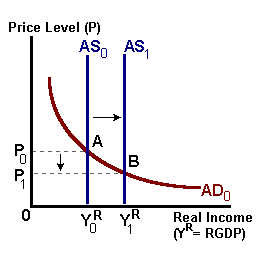
In the aggregate economy the price level is determined by the balance (or imbalance) between the ability to produce goods and services and the ability to spend to acquire those same goods. The ability to produce is summarized by the long run aggregate supply (AS) function based on the level of technology and availability of factor inputs (see the 'Concept' opener). The ability to spend is summarized by the aggregate demand (AD) relationship which represents combinations of income and interest rates such that product markets and financial markets are in equilibrium. As prices rise, purchasing power falls, and thus the quantity of goods and services that can be acquired with a given nominal income declines. Aggregate Demand represents this inverse relationship between the price level and purchasing power.

Long-run Aggregate Supply shifts

A supply-side shock, such as an increase in labor productivity, would shift AS outward -- there is now a greater potential to produce at each and every price level. We can see this change in the figure above. This shock, in time, creates an excess supply of goods (Y* > Y^R) and puts downward pressure on the price level. As prices fall, purchasing power increases reflecting an increase in the ability to spend (i.e., a movement from A to B). The net result is an increase in output and spending and a lower price level.

In the figure below we have a demand-side shock perhaps the result of an increase in government spending or lower interest rates. This shock shifts the AD relation outward. Initially there is an excess demand for goods (A to B) evidenced by a depletion of inventories. Given that potential output has not changed, in time this excess demand will cause the price level to increase. As prices increase, purchasing power falls and the ability to spend decreases (B to C). The net result of this shock is an increase in the price level with no change in output or real spending.

An expansionary shift in Aggregate Demand

9.2.1 Price Adjustment and the Real GDP / Output Gap

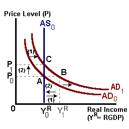
The process of price adjustment is a bit more complicated than just moving to a new intersection in our AD-AS model. There are a series of events and linkages that tie changes in prices to unemployment and wage changes, output gaps and unemployment, and the markup of prices over production costs. We will outline this below.

1. The Markup Given that wages are a large part of national income and thus represent the bulk of production costs, changes in prices are often strongly related to changes in wages as actual output falls short of (or exceeds) potential output. Thus:

Costs = f(wages)

and

Prices = α[Costs]

where 'α' is some markup factor (α > 1.0) dependent on the ability of business firms to pass cost increasess onto the consumer. The above two relationships allow for the establishment of a relationship between the level of output and changes in the price level.

The Phillips Curve

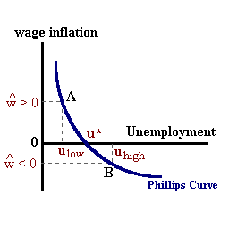
2. The Phillips Curve In 1958 A.W. Phillips established an empirical relationship (the Phillips Curve) between wage inflation and the gap between the actual level of unemployment 'u' and the natural rate of unemployment 'u*'. A rate of unemployment 'u_high' above this natural rate would imply slack in labor markets such that wages would be expected to fall. A rate of unemployment 'u_low' below the natural rate would signal tight labor markets such that wages are being bid upwards as employers attempt to fill out the ranks of their required labor force. The parameter 'b' represents that rate at which wages adjust to tightness or slack in labor markets.

%Δw = -β(u - u*)

if u > u* then

%Δw < 0

and wage deflation exists. Otherwise if u < u*,

%Δw > 0,

we have wage inflation.

Okun's Law

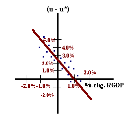
3. Okun's Law A third empirical relationship is Okun's law which states that for every percentage point 'u' exceeds 'u*', growth in Real GDP is 2.5% below the rate of growth in potential output in the U.S. economy.

%ΔY^R - %ΔY* = -2.5(u - u*)

This expression can be rewritten as:

(u - u*) = Φ(%ΔY^R - %ΔY*)

where Φ = - (1 / 2.5).

Finally given our markup equation:

Prices = α(wages) or %ΔP = α(%Δw)

i.e., price inflation is related to wage inflation, we can develop the following relationships:

%Δw = -β(u-u*)

and

(u-u*) = -Φ(%ΔY^R - %ΔY*)

or

%ΔP = α[-β(-Φ(%ΔY^R - %ΔY*)]

or given:

Θ = α(-β)Φ,

%ΔP = Θ(%ΔY^R - %ΔY*)

In this final expression, we find that changes in the price level are related to the difference between the ability to buy goods and services in a particular economy Y^R and the ability to produce those goods and services Y* -- prices changing in reaction to gaps between potential output and Real GDP. If:

%ΔY^R_t > %ΔY*

then

%ΔP > 0

and inflationary pressure exists in the economy. If the opposite is true, we will then observe deflationary pressure in the economy.