Douglas A.Ruby
Life-Cycle Hypothesis
Aggregate Demand
Aggregate Expenditure
Macroeconomic Theory
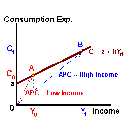
Early Keynesian models of the consumption function related current consumption expenditure to current levels of income or disposable income. These models took the form of:
C = a + bYdSeveral theoretical implications can be developed by taking the ratio of consumption expenditure to the level of disposable income. This ratio known as the 'APC' the average propensity to consume eliminates the need to convert nominal values into their real counterpart in that changes in the price level cancel out:
whereC = Consumption Expenditure
a = Autonomous consumption
consumption expenditure independent of the level of income.
b = the Marginal Propensity to Consume 'MPC'
which represents the fraction of each additional dollar of income
devoted to consumption expenditure.
and
Yd = Current Disposable Income.
APC = Real Consumption
Real Income= Nominal Consumption / P = Nominal Consumption
Nominal Income/P Nominal Income
Thus the APC can be computed by dividing both sides the the Keynesian consumption function by disposable income:
APC = C/Yd = a/Yd + b(Yd/Yd)or
APC = a/Yd + MPC.

Given this final result we can look at the theoretical implications of the Keynesian consumption function over a different income groups (the cross- section) and over time (a time series). For the cross-section we would expect that lower-income groups would consume a greater proportion of their income relative to high-income groups:
APClow income > APChigh income
With time series data we would expect that over time and as disposable income increases the APC should decline:
APCt-1 > APCt > APCt+1
It is in this latter case that this particular consumption function fails to explain real world behavior. In empirical studies, the APC is observed to be smaller for higher income groups relative to low income groups. However, over time the APC is observed to be constant independent of growth in aggregate measures of income. This failure led to the development of alternative theories of the consumption function one of which is the Permanent Income Hypothesis or 'PIH'.
The PIH begins to explain consumption behavior by first redefining measures of income. Observed values of aggregate income 'Y' can be divided up into two separate components: 'YP' Permanent (or projected levels of) Income and 'YT ' Transitory (or unexpected changes in) Income. Thus:
Y = YP + YT.
The transitory component has an expected value of zero (E[YTt] = 0) reflecting the notion that over time transitory gains are offset by future transitory losses and vice-versa. Thus in the long run observed levels of income 'Y' are equal to permanent income 'YP'.
Finally, according to the PIH consumption expenditure is proportional to permanent income:
C = kYP
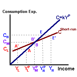
such that the parameter 'k', a constant, represents both the average propensity to consume and the marginal propensity to consume. This consumption function (as shown with the blue line below) is described more accurately as a long run consumption function consistent with the observed long run results of consumption behavior.
Observed short run behavior is explained through the value of transitory income for different income groups. Specifically, transitory income for low income groups is assumed to be negative reflecting the notion that over time transitory losses exceed transitory gains for this group of individuals:
YTL < 0 => YL < YPL
For middle income groups the value of transitory income is equal to zero over time such that observed and permanent income take the same value:
YTM = 0 => YM = YPM

Finally, for high income groups, transitory gains exceed transitory losses such that transitory income is on average positive over time or:
YTH > 0 => YH > YPH
The impact of this transitory component can be used to develop a short run consumption function (the red line) as shown in the diagram.

|

|

|