Usually, we study the behavior of the markets using the traditional supply and demand framework. This type of analysis of market conditions is called partial equilibrium analysis where we look at the determinants of price and quantity in a particular market holding all other markets constant.

A natural extension to the above type of analysis is general equilibrium analysis or how demand and supply conditions interact in several markets to determine the price of many goods. A common tool in general equilibrium analysis is the Edgeworth boxwhich allows for the study of the interaction of two individuals trading two different commodities. Production is taken as a given and represented by an initial endowment of goods in possession of the two individuals . This type of analysis draws on the use of indifference curve analysis and consumer preferences to analyze trading outcomes.

Figure 1, the Edgeworth Box

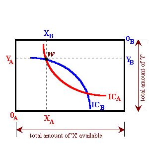
The lower left-hand corner represents the origin for consumer 'A' and the upper right-hand corner represents the origin for consumer 'B'.  Person A's preferences (indifference curves) are convex to the origin O_A. Person B's preferences are convex to O_B.

Moving to the right means that person 'A' has more of commodity 'X' and person 'B' has less of that commodity. Moving upwards means that person 'A' has more of commodity 'Y' and person 'B' has less. Moving in the northeast direction makes person 'A' better off. Moving in the southwest direction makes person 'B' better off.

Rather than introduce budget lines for the two consumers, the Edgeworth box uses the concept of initial endowments. An initial endowment 'ω' represents the amount of commodities X & Y individuals A & B have available before trade. Thus (X_A ,Y_A ) =  w_A and (X_B , Y_B ) =  w_B where w_A and w_B represents A's and B's initial endowments (or income). The height of the Edgeworth box represents the total amount of commodity 'Y' available and the width of the Edgeworth box represents the total amount of commodity 'X' available. In the absence of any production, the dimensions of the box remain constant.

One goal of general equilibrium analysis is to determine if it is possible to make individual 'A' and/or individual 'B' better off through the process of exchange given their initial endowments. For example a trade such that these two individuals move to point 'R' in the diagram below would make person 'B' better-off with out harm to 'A':

Figure 2, the Negotiation Space

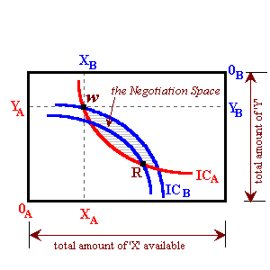
Any trade that puts these two individuals into, or on the border of, the shaded area will make one or both individuals better off. This is known as a Pareto Improvement. As long as any Pareto Improvements remain, an incentive for trade exists between these two agents.

An optimal allocation of commodities is determined by the concept of Pareto optimality. A Pareto optimal allocation of commodities is that allocation where it is not possible to make one person better off without making any other person worse off. This is shown graphically in the diagram below where the indifference curves of person 'A' are just tangent to person 'B' as occurs at point 'T'.

Figure 3, A Pareto Optimum

If, for example, the two consumers are at the initial endowment point 'w', it is possible to make person 'B' better off by moving to point 'R' without making person 'A' worse off (a movement along person A's indifference curve). A second trade could be the movement towards point 'T' which would make person 'A' better off without making person 'B' worse off.  This trade (from w to T) would make both person 'A' and person 'B' better off.

You might remember that the slope of an indifference curve dy/dx is just the ratio of the marginal utilities of goods 'X' & 'Y' (or: dy/dx = MU_x / MU_y = MRS_xy) thus the condition for Pareto optimality may be properly defined as that point where:

MRS^A = MRS^B .

The next step in general equilibrium analysis is the determination of how this movement actually takes place from the initial endowment to a Pareto efficient allocation. This movement is acomplished through the price system where the relative prices between goods 'X' & 'Y' represent the terms of trade between the two individuals. The slope of any line passing through the endowment point represents this price ratio of commodity X and commodity Y. Thus if that line is relatively steep, commodity X is relatively more expensive than commodity Y. If the line is relatively flat, then the opposite is true.

Through some hypothesized auction process (where different price ratios are called out), a market or competitive equilibrium will be established at that point  (a Pareto Optimum), where:

MRS^A_xy = (MUⁱ_X / MUⁱ_Y ) = MRS^B_xy = (P_x / P_y )   for   i = A,B