 |
 |
The key to understanding investment decisions is the determination of K*, the desired capital stock. This desired level is based, as stated above, on profit-maximizing behavior of the firm. There are several methods by which we can approach the profit-maximizing level of capital stock. First, we can analyze the net present value of different amounts of capital to determine which quantity gives the greatest discounted stream of profits. For example, given the following:
With this data we will use the following annuity factor computation:
PVn = (Revenue)[1 - (1 + r)-n] / r
= (Revenue) [1 - (1.05)-10] / 0.05 = (Revenue) 7.722
K Output
(units)Revenue PV
(n=10)less Costs
[Pk(K)]Net Present Value 1 50 $250 $1930.50 $1000 $930.50 2 90 $450 $3474.90 $2000 $1474.90 3 120 $600 $4632.00 $3000 $1632.00 4 140 $700 $5405.40 $4000 $1405.40 5 150 $750 $5791.50 $5000 $791.50
In the above example (assuming diminishing marginal productivity) we find that three units of capital would generate the greatest net present value and thus the greatest profits.
A second approach is the marginal approach where we compare the contribution to revenue by using one more unit of capital with the costs of acquiring that unit of capital. The contribution to revenue is known as the Marginal Revenue Product (MRP) of capital and is calculated by multiplying the marginal product with the market price of the output produced:
MRPk = MPKPx
The contribution to costs is known as the Rental Cost of Capital (RCC) which includes borrowing costs (or opportunity costs of using internal funds for investment expenditure) and depreciation costs:
RCC =PK(r) + PK(δ) = PK(r + δ)
We will use similar data and a table for an example:
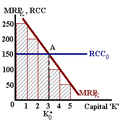
| K | Output | MPk | MRPk | RCC (r = 5%, δ = 10%) |
| 1 | 50 units | 50 | $250 | $150 |
| 2 | 90 | 40 | $200 | $150 |
| 3 | 120 | 30 | $150 | $150 |
| 4 | 140 | 20 | $100 | $150 |
| 5 | 150 | 10 | $50 | $150 |
If the MRP exceeds RCC then profits will increase by acquiring additional units of capital (contribution to revenue exceed contribution to costs). If the opposite is true then the additional costs associated with one more unit of capital exceed the revenue generated and profits will decline.
Similar to the Net Present Value approach, we find that with three units of capital the contribution to revenue of the third unit is just equal to the costs of acquiring and using that third unit--profits will be a maximum at this level of input as shown in the diagram below-left.
|
|
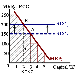
A change in interest rates would increase the rental cost of capital 'RCC' such that this third unit is no longer profitable. The firm would react to this cost increase (an increase in the price of capital would have similar effect), by using less capital in production. This is shown in the above diagram-right.
A third approach is using a calculation similar to the present value of a perpetuity (again, see the. We begin by using the marginal conditions above:
Marginal Revenue Product = Rental Cost of Capital
MPKPx = PK(r + δ)
And we rearrange the terms:
[MRPK - PK (δ)] / PK = 'Ψ'
This term Ψ represents the yield on the last unit of capital employed in the production process:
| K | Output | MRPK - PK (δ ) | PK | Yield |
| 1 | 50 units | $250-$100 | $1000 | 15% |
| 2 | 90 | $200-$100 | $1000 | 10% |
| 3 | 120 | $150-$100 | $1000 | 5% |
| 4 | 140 | $100-$100 | $1000 | 0% |
| 5 | 150 | $50-$100 | $1000 | NA |
In this case, we find that the yield on the first two units of capital is greater than the market interest rate and thus may be acquired to earn profits over-and-above the borrowing costs. It is the third unit of capital where the yield is just equal to the market rate of interest -- no additional profits may be earned by hiring additional capital.
In all three approaches we find that the desired capital stock 'K*' is equal to three units based on the productivity of capital, the rate of depreciation, the price of capital and the output being produced and, of greatest importance, market interest rates.
We can use a Cobb-Douglas form of the production function to solve for K* and combine this with the expression for investment defined above:
Xoutput = ALαKβ and MPk = βX/K
given MRPk = RCC,
β(X/K)Px = Pk(r + δ)
or
K* = [β(Px)X] / [Pk(r + δ)]
Inserting this expression for K* into the investment expenditure equation gives us:
It = Pk{[β (Px)X] / [Pk(r + δ)] - (1 - δ)Kt-1}
or
It = [β (Px)X] / (r + δ) - (1 - δ)PkKt-1
where we find that Investment is inversely related to market interest rates and the price of a unit of capital, positively related to output prices and the productivity of capital (as measured by the parameter ' β, and undetermined with respect to the rate of depreciation.
Aggregating over all investment expenditure equations for all firms we can write the following simplified expression:
I = I0 - h(r)
where I0 captures the effects of changes in the price of capital, the rate of depreciation, and the price level. The parameter h is known as the interest sensitivity of investment capturing the inverse relationship between investment expenditure and real interest rates.
|
|