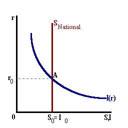
An Increase in Investment expenditure
Before After
A general approach to analyzing changes in the structure of interest rates, and more specifically the real interest rate is via the Flow of Funds model. This model examines the broad determinants of savings in a macroeconomy and treats the real interest rate as the variable that aligns a given level of savings with investment needs.
Savings represents the source of funds in the model and domestic Investment Expenditure represents the use of those funds. It is important to keep in mind that these funds being transferred from lender to borrower represent scarce resources. These resources are made available via the saver foregoing current consumption allowing these resources to be used for the creation, accumulation, and replacement of capital -- capital that will allow labor to be more productive in the future.
The model begins with the Income Identity:
Y = C + I + G + NX
rearranging terms:
Y - C - G - NX = I(r)
where the left-hand-side of the equation represent the source of funds and the right-hand-side, the use of funds. Additionally, we note that Investment decisions are (negatively) related to the real rate of interest 'r'.
By subtracting and adding-in taxes 'T' which represents the transfer of resources from the private sector to the public sector we have:
[Y - T - C] + [T - G] + [-NX] = I(r)
Each term in brackets now represents a separate type of savings defined as follows:
Note that NX represents the Current Account Balance component of the balance of payments. Thus, its negative, [-NX] represents the Capital Account Balance
Adding these three terms together we have:
SNational = Spvt + Spub + Sforeign
This is shown by the vertical line in the diagram below. The real rate of interest will adjust in competitive financial markets to bring National Savings into an equality with Domestic Investment as shown by ro.This vertical line indicates that the aggregate level of savings is independent of the real interest rate. This may or may not be true. Empirical studies indicate that aggregate savings may be highly inelastic although not perfectly inelastic. For purposes of our graphical model the net effect on real interest rates is the same with individual shocks leading to increasese or reductions in this real rate.
Various shocks can affect the flow of funds and thus the rate of interest. For example, an increase in investment expenditure perhaps due to an increase in the productivity of capital or due to growth in the real economy will shift the Investment schedule to the right

The net effect here is an increse in the real interest rate.
Fiscal policy shocks can also affect the flow of funds and real interest rates. For example, suppose that Government Expenditure G decreases. Holding taxes constant, this will lead to an increase in Public Savings and National Savings The savings function will shift to the right creating an excess supply of funds thus causing the real rate of interest to fall

 Tax Rate
Changes to the tax rate is a bit more complicated. Changes in taxes affect both consumption expenditure and thus Private Savings as well as Public Savings directly. However, working through the marginal propensity to consume, a decrease in the tax rate reduces Consumption Expenditure / Private Savings by more than the increase in Public Savings. The net effect, in this model, is an increase in the real interest rate.
A Numerical Example
Suppose that we have the following equations:
C = 0.80(Y - T) ... consumption expenditure, MPC = 0.80
T = 0.20(Y) ... Tax Revenue, tax rate = 20%
G = 2,000 ... Government Exp. (billions)
NX = -500 ... Current Acct. Balance (deficit)
I = 2,600 - 100(r) ... Investment Exp.
Y = 10,000 ... Real GDP (Output in billions) held constant.
Solving (given Y = 10,000), we find that:
T = 2,000
C = 0.80(10,000 - 2,000) = 6,400
and
Spvt = Y - T - C = 1,600,
Spub = T - G = 0 and,
Sforeign = [-NX] = 500
thus,
SNational = 1,600 + 0 + 500 = 2,10
setting SNational = I(r) we have:
2,100 = 2,600 - 100(r) and
r0 = 5% and Investment expenditure = 2,100.
Now, if the tax rate were to be reduced to 10% (t' = 0.10):
T' = 1,000
C' = 0.80(10,000 - 1,000) = 7,200 and
Δ C = +800
and
S'pvt = Y - T - C = 1,800 and
Δ Spvt = +200
S'pub = T - G = -1,000 and
Δ Spub = -1,000
Sforeign = [-NX] = 500 as before.Thus,
S'National = 1,800 - 1,000 + 500 = 1,300 and
Δ SNational = -800setting S'National = I(r) we have:
1,300 = 2,600 - 100(r) or
r1 = 13% and
Investment expenditure = 1,300.Reducing the tax rate from 20% to 10% has led to an increase in the real interest rate from 5% to 13%. With this interest rate increase, private Investment Expenditure will be reduced (from 2,100 to 1,300).
We must note that the outcome in this example is only looking at the demand-side of the aggregate economy and the source of loanable funds. It can also be the case that the reduction in tax rates may increase the after-tax return on capital leading to more investment demand.